Correlating Multiple Wireshark Captures: Follow the Same Packet Across the Network

So many times I have watched YouTube videos and read articles that jump right into Wireshark troubleshooting of multiple captures of a network conversation or event from multiple points in the network. To me, that can be unnecessarily overwhelming to those learning packet capture. In many videos, it never becomes clear why two different capture points were even needed. Frankly, it is hard to watch.

The concept of following a packet across a network is an important one. So let’s take a step back. Consider the following very simple network:

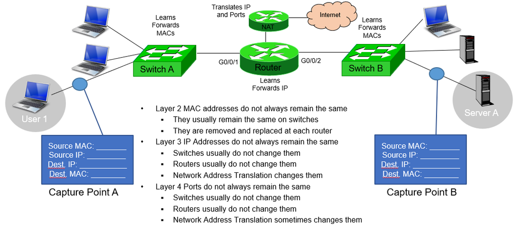
Can you fill in the Addressing blanks?

On Capture Point A, they will be as follows:

• Source MAC: User 1 Interface
• Source IP: User 1 IP Address
• Destination IP: Server A IP Address
• Destination MAC: Router G0/0/1 Interface

On Capture Point B, they will be as follows:

• Source MAC: Router G0/0/2 Interface
• Source IP: User 1 IP Address
• Destination IP: Server A IP Address
• Destination MAC: Server A Interface

It becomes clear that the packets change as they travel across the network through various nodes.

So consider the challenges of correlating these two packet captures. If you are new to packet capture, I urge restraint in capturing in multiple places because of the challenges and complexities involved with packet capture correlation.

In practical troubleshooting, most network problems can be diagnosed from a single, well-chosen capture point. If you capture close enough to the problem and you understand what that vantage point can and cannot see, one trace will often reveal TCP behavior, DNS failures, retransmissions, resets, latency, application response timing, ICMP errors, routing symptoms, MTU problems, and many other issues. In many cases, adding more capture points just adds complexity without improving the diagnosis.

Multiple captures become valuable when the question is specifically where along the path something changed or disappeared. That is when you need to compare what entered a device or network segment with what came out of it. Examples include proving a firewall dropped traffic, identifying where NAT or encapsulation changed a packet, locating where latency was introduced, or comparing wireless and wired behavior across an access point.

That said, I fully recognize that when troubleshooting a difficult and complex network problem, one packet capture does not always tell the whole story. A capture taken at the client tells you what the client transmitted and received, but it cannot necessarily tell you what happened after that traffic passed through a router, firewall, wireless access point, WAN, load balancer, or other network device. These intermediate nodes can create a number of problems along the way.

In these types of scenarios, sometimes the best way to answer the question is to capture the traffic at two or more locations.

For example, imagine capturing on both sides of a firewall:

Client ---- Capture A ---- Firewall ---- Capture B ---- Server

If a packet appears in Capture A but never appears in Capture B, you have learned something important.

Likewise, if the packet appears at both locations but has been changed in some way we do not expect, delayed, fragmented, encapsulated, translated, or reordered, comparing the two captures can provide evidence that would be impossible to obtain from either capture individually.

But this introduces a new challenge: How do you prove that a packet in Capture A corresponds to a packet in Capture B?

That is the process I refer to as packet capture correlation.

Correlation Is More Than Merging Two PCAP Files

Wireshark can merge capture files, and the mergecap utility can do the same thing from the command line.

But merging two files does not automatically correlate them:

• If the clocks on the capture devices differ, the packets may appear in the wrong chronological order
• If the same packet was captured at two locations, the merged trace may contain two copies of it
• If a router or firewall modified the packet along the way, the two copies may not even look identical

In some situations, merging the files can actually make troubleshooting more confusing and overwhelming.

Before combining captures, I prefer to answer a more fundamental question:

What evidence can I use to determine that these two packets represent the same network event?

Once that relationship is established, timestamps become only one part of the analysis.

What Can Be Used to Correlate Packets?

There is rarely a single perfect identifier. Instead, I usually look for a combination of characteristics. Useful correlation points include:

• source and destination IP addresses
• source and destination TCP or UDP ports
• TCP raw sequence and acknowledgment numbers
• TCP flags
• IP identification values
• packet or payload length
• ICMP identifiers and sequence numbers
• DNS transaction IDs and query names
• application transaction identifiers
• distinctive payload contents using the “contains” display filters
• VLAN, VXLAN, GRE, or tunnel information
• recognizable request/response sequences
• timestamps and relative timing

The stronger the combination, the more confidence you can have that you are looking at the same packet or transaction.

TCP Sequence Numbers Are Particularly Useful

TCP traffic gives us some excellent correlation information.

Imagine seeing this packet near the client:

192.168.1.100:51522 → 203.0.113.20:443

SEQ = 352104
ACK = 819223
TCP Payload = 1460 bytes

You then find a packet near the server containing the same TCP sequence number, acknowledgment number, payload length, and conversation information.

That is strong evidence that you have found the same TCP data.

Even if some Layer 2 or Layer 3 information changed between the two locations, the TCP information can still provide a useful fingerprint.

But be careful. A retransmitted TCP segment can have the same sequence number and payload length as the original packet. Sequence numbers alone may therefore not uniquely identify one physical transmission.

Correlation is about using multiple pieces of evidence together.

Don’t Expect the Packets to Be Identical

One of the most important lessons in multi-point analysis is that the same packet may look different at different observation points.

Consider a packet crossing a router:

Capture A                     Capture B
---------                     ---------

Ethernet A                    Ethernet B
IPv4 TTL = 64                 IPv4 TTL = 63
IP checksum A                 IP checksum B
TCP                           TCP
Payload                       Payload

The Ethernet headers should change because the packet has moved onto another Layer 2 network.

The IPv4 TTL changes because the router decrements it. The IPv4 header checksum must therefore change as well.

Yet the TCP segment and application payload may still be effectively the same.

So attempting to correlate packets by comparing every byte would fail.

You have to understand which fields should remain stable and which fields are expected to change.

NAT Makes Correlation More Interesting

Now place a NAT router between the two capture points.

Capture A might show:

192.168.1.100:51522 → 203.0.113.20:443

while Capture B shows:

198.51.100.50:62001 → 203.0.113.20:443

Both the source IP address and source TCP port have changed.

If you search the second capture only for:

192.168.1.100

you will never find the packet.

Instead, you may need to correlate using TCP sequence numbers, ACK numbers, payload size, application information, timing, and your knowledge of the NAT translation.

This is exactly why multi-point packet analysis requires more than simply comparing Source and Destination columns.

Tunnels Can Change the Packet Even More

GRE, VXLAN, IPsec, and other tunneling technologies introduce another level of complexity.

Before encapsulation you might have:

Ethernet
IPv4
TCP
Payload

After encapsulation:

Ethernet
Outer IPv4
UDP
VXLAN
Inner Ethernet
Inner IPv4
TCP
Payload

The packet looks radically different.

But the inner packet may still provide the evidence needed to correlate what entered the tunnel with what came out.

This is one reason the Wireshark # Layer Operator (which you can read more about) can be so useful. It allows us to distinguish fields such as:

ip.src#1

from:

ip.src#2

when multiple instances of IP exist within the same captured frame.

Correlation often requires understanding encapsulation rather than merely matching addresses.

Wi-Fi to Ethernet Is Another Great Example

Suppose you capture a client transmission using monitor mode while simultaneously capturing the traffic leaving the access point on Ethernet.

The wireless packet may contain an 802.11 header:

802.11
LLC
IPv4
TCP
Payload

while the wired capture contains:

Ethernet
IPv4
TCP
Payload

There isn’t an identical frame on both sides. The access point has bridged the traffic between two different Layer 2 technologies. So don’t try to correlate using the Ethernet or 802.11 headers. Move farther up the protocol stack. The IP addresses, TCP information, application data, and timing may provide much better evidence.

This is a general rule I use frequently:

If a field can legitimately change between the two observation points, don’t make that field the foundation of your correlation.

Deliberately Create a Correlation Marker

If you know in advance that you will be capturing at several locations, you can make your life much easier by deliberately generating recognizable traffic.

For example, immediately after starting the captures you could generate a unique:

ping

DNS request:

correlation-test-0912.example

HTTP request, TCP connection, or another easily identifiable transaction.

Then generate another recognizable event before stopping the captures.

You have essentially created bookends for your captures.

Those events can help you establish:

• which capture began first
• approximate clock differences
• whether clock drift occurred
• whether the same traffic is visible at every observation point

This becomes particularly useful when captures run for a long time.

Time Is Evidence, But Don’t Trust It Too Quickly

Timestamps are extremely useful for correlation. But they can also be dangerous.

Suppose the same packet appears in:

Capture A: 10:00:00.100

Capture B: 10:00:00.125

It is tempting to conclude:

The packet took 25 milliseconds to travel between the two capture points.

Maybe.

But that 25 milliseconds could contain:

Actual network transit time
+
Clock offset
+
Clock drift
+
Capture-system timestamping differences

Without synchronized clocks, you cannot automatically attribute the entire difference to the network. This becomes especially important when using two PCs to perform the captures. Their clocks may look identical to you while differing by tens or hundreds of milliseconds—or much more.

Clock Offset and Clock Drift Are Different

There are actually two clock problems.

A clock offset means one system might consistently be two seconds behind another.

Conceptually:

Capture A     Capture B

10:00:00      09:59:58
10:10:00      10:09:58
10:20:00      10:19:58

The difference remains approximately two seconds.

But clock drift means the difference changes:

Beginning     1.2 seconds
Middle        1.8 seconds
End           2.5 seconds

Simply adding two seconds to every packet won’t fix that. Wireshark has a little-known Time Shift capability that can use two timestamp reference points and linearly correct clock drift across an entire capture.

I’ll cover that technique separately because it deserves a discussion of its own.

Sometimes You Shouldn’t Merge the Captures

This may be the most important point in this post. There is a natural temptation to think:

Two PCAP files are inconvenient. I’ll merge them and then analyze one file.

That is not necessarily better.

Suppose Capture A and Capture B both contain the same TCP segment. The merged capture now contains:

TCP Segment at Capture A
TCP Segment at Capture B

Wireshark’s TCP analysis sees packets in a single trace. It does not inherently understand that those two packets represent the same transmission observed at two different locations.

That can affect your interpretation of:

• retransmissions
• duplicate ACKs
• out-of-order packets
• TCP timing
• RTT measurements
• Expert Information

What looks like duplicate network traffic may simply be duplicate observation.

For some investigations, keeping two Wireshark windows open side-by-side is far cleaner than merging the captures.

My Preferred Workflow

When I am correlating captures from multiple observation points, I generally think about the process in this order:

Understand the capture locations
            ↓
Identify common traffic or events
            ↓
Determine what fields should remain unchanged
            ↓
Determine what fields should change
            ↓
Match several packets or transactions
            ↓
Compare the timelines
            ↓
Determine clock offset or drift
            ↓
Decide whether timestamps require correction
            ↓
Decide whether merging actually helps
            ↓
Perform the analysis

Notice that: Merge the captures is not Step 1. Sometimes it never happens at all.

Preserve the Original Captures

Whenever you modify timestamps, remove packets, merge traces, or otherwise manipulate capture files, preserve the originals.

I like using names that make the distinction obvious:

client-original.pcapng
server-original.pcapng

client-time-corrected.pcapng

client-server-merged.pcapng

That way there is never any question about which file contains the original evidence and which contains modifications made for analysis. This is good troubleshooting discipline even when the capture isn’t associated with a security or forensic investigation.

The Real Goal Is to Follow the Packet

Multi-point packet analysis can answer questions that a single capture simply cannot.

• Did the packet leave the client?
• Did it reach the router?
• Did the firewall forward it?
• Was NAT applied?
• Did it enter the tunnel?
• Did it emerge from the tunnel?
• Did the server receive it?
• When did the response come back?
• Where was the delay introduced?

Those questions require something more sophisticated than opening two PCAPs and looking at their timestamps. They require correlation. And once you start thinking in terms of correlating packets rather than merely merging capture files, multiple-capture troubleshooting becomes much more useful—and much less likely to lead you to the wrong conclusion.

So, what if the packets correlate correctly, but the capture clocks don’t? In my next advanced Wireshark tutorial, I’ll look at Wireshark’s Time Shift feature—including its ability to use two known timestamps to correct clock drift across an entire capture before you merge or compare the files.

---

If you would like to help support the continued development of independent networking, broadband, Wi-Fi, VoIP, and packet analysis content, please consider joining our Patreon community where you will gain access to exclusive technical resources, downloadable labs and PCAPs, bonus course content, troubleshooting guides, and additional member-only material.  Comments and technical discussion are always welcomed at our Patreon community or on our Discord server.  You can also support our work by simply buying us a coffee — every contribution helps us continue creating practical, real-world network science education for professionals and enthusiasts alike.